Saturday, April 12, 2008

Villarceau Circles and Diagonal Rotation of RPM Map

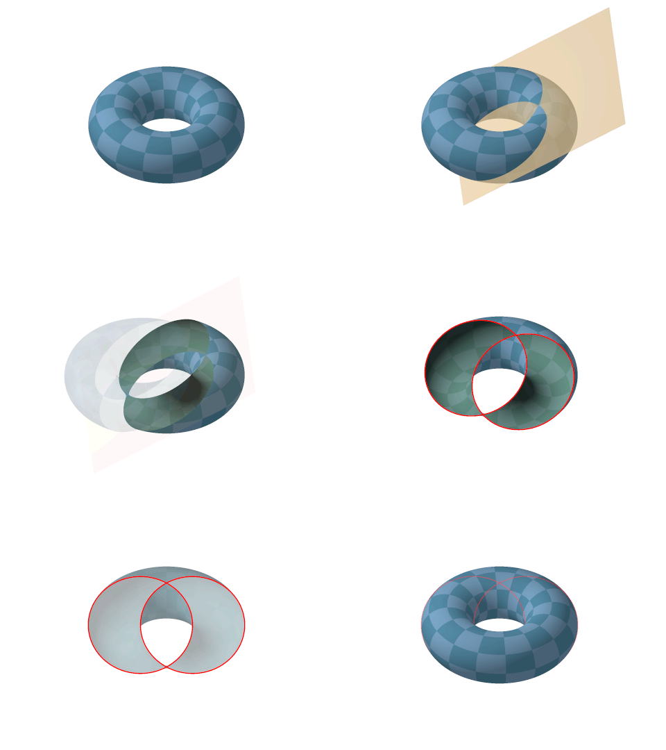
It has been known for long time that there are 4 perfect circles passing every points on the a torus surface. We can get two of these circles buy cutting the torus vertically and horizontally through that points. These two circles are the normal circles most people can easily visualize. The other two, not so apparent, circles are the so-called Villarceau circles. They are made by cutting the torus diagonally as depicted in the following animation (IE7 users need to enable the flag Tools>Internet Options>Advanced>"Play animations in web pages" to see the animation):
Villarceau Circles Animation
Figure 1: Creating the Villarceau Circles on a torus.


Above animation is very helpful to visualize the Villarceau Circles. Another simple way to show the Villarceau circles is using the fundamental polygon representation where a torus is represented as a rectangle whose opposite edges are glued together. In the polygon represetnation, the horizontal and vertical edges are the two normal circles (horizontal and vertical circles). The two diagonals are the Villarceau circles as depicted in the following diagram:


Figure 2: Four circles on a torus passing through a point.


We know that RPM algorithm simulates a multi-particle dynamic system confined on the flat torus surface. For some unknown reasons, RPM maps often form symmetry patterns alone the diagonal lines, e.g. along the Villarcea circles. For instance, when we map the sphere to the tours, RPM algorithm cuts the sphere into two equal sized half and map them as two discs to the torus surface. The two discs are positioned alone a a diagonal line as depicted in the following picture:


Figure 3: RPM Map of a sphere


We see in above picture that only one disc is completely displayed as a whole, the other one has been cut by the edges into 3 or 4 pices (which will form a complete disc when we glue the opposite edge together). The whole picture is more or less symmetric with respect to the left-up-to-right-bottom diagonal line. We can get a better visualization of above image when we tile multiple copies of above map together as be show in the following picture:


Figure 4: Tiling duplicates of Figure 3.


Now, it would be helpful for the purpose of visualization if we can show the two discs as whole discs in a single map without using the tiling techniques. We can achieve this by transforming the coordinator from the two vertical and horizontal edges to the two diagonals (i.e. the two Villarceau circles). The transformation is schematically depicted in the following diagram:


Figure 5: Rotation to the diagonal circles.


We call the above transformation the diagonal rotation as it basically rotate the coordinator to the diagonals. Formally, the diagonal rotation is done by the following forms:


In above forms w and h are the width and height of the fundamental rectangle respectively. d is the length of its diagonal. The above forms transforms points from the region D to D'. For points from other regions, we have to apply some simple shifting after the transformation as indicated in Figure 5.

As indicated in Figure 5, the two diagonals will become the edges of the transformed map. Thus, in order to avoid the resulting map be cut off by the edges we should shift a RPM map away from the diagonals through torus cyclical shifting. For our sphere example we can shift the map, for instance, to the following position:


Figure 6: Sphere map shifted off from the diagonal lines.


When we now apply the diagonal rotation on the map in Figure 6 we will get the following rotated map:

Figure 7: The sphere map after diagonal rotation.

Comparing with the original RPM map in Figure 3, the rotated map in figure 7 is obviously easier to investigate for human eyes.


It should be pointed out that a RPM map after diagonal rotation is no long a torus map in the sense that you cannot tile the map to fill 2D space the same way as be shown in Figure 4. Since this will break the edge-connectivity as indicated in Figure 5. But you can fill the 2D space with the rotated RPM map like building a bridge wall: you tile the map site by site to build a continuous lay, then build next lay the same while shift the lay to the left (or right) for half block. The following picture depicts this characteristics:


Figure 8: Tiling with rotated map.

Friday, April 4, 2008

The Equivalence of Cooling and Expanding Dynamics

The RPM (relational perspective map) algorithm has a seemly add-hoc measure that gradually decreases the learning rate to force the convergence of the algorithm. I have tried to avoid such measure with various methods (e.g. conjugated algorithm exploring second order gradient), but was not able to find anything working.

I have notice a significant problem here: In the original Newton-Raphson algorithm, the algorithm should converge to a local minimum if the learning rate is sufficiently small. But, this not so for the optimization problem of RPM. The algorithm never converges, no matter how small the learning rate is (in a way that is doable with double precision arithmetic). If I keep the learning rate constant at certain small value, the simulated dynamic system goes in to an equilibrium state with constant variance.

Thus, it looks like NR method, as it is, does not work for massively complex dynamic system, it is not stable enough. Letting the learning rate gradually vanish seems to be the simplest method to enforce the convergence.

Mathematically, a very fine granulated gradient descent algorithm should be able to find a local minimum. But, I think this is practically not possible. To understand this, we notice that the learning rate practically controls the average variance of the positions of the simulated particles. That means, the learning rate is a kind of "temperature" of the system. In physics, we know that if we keep the temperature constant, the system will never converge to a frozen state. We can only reach that state when we gradually reduce the temperature to zero.

It is interesting to notice that the cooling dynamic system simulated by RPM is theoretically equivalent to a n-body dynamic system that is ever expanding. To see this, we notice that the learning rate is directly linked to the average variance of the particle's positions. Thus, instead of gradually lowering learning rate, we can just reduce the scale of unit length of the space compared to total size of the space (e.g. the size of the torus). The latter is again equivalent to a system in which we keep the scale of unit length constant, but gradually expand the size of the whole space.

We see here certain similarity of RPM model with the inflationary big-bang model from cosmology. Whereas RPM keeps the total size of the system stationary and gradually reduces the energy, the big-bang model keeps the total energy constant but let the universe expands. It is probably not a too crazy idea to consider a dual big-bang model that keeps the apparent universe stationary, but magically reduces the total energy/mass/temperature.