Multidimensional Sorting with High Fidelity t-SNE

 Multidimensional Sorting with High Fidelity t-SNE

Multidimensional data often has a latent sequential structure that determines the basic shape of the data. Those sequential structure might correlate with ordered quantities like time, stages and size etc. Capturing and visualizing those sequential structure would be very helpful for exploratory data analysis.  

A frequently used method for exploring high dimensional data is the principal component analysis (PCA). By projecting data to the main principal components, we can gain institutive information about the high level large scale shape of the data. More particularly, the projection to the first principal component offers a way to visualize the main back-bone linear structure.

A main short-coming of PCA is that it only structure from linear perspective. It fails for data whose latent sequential structure significantly deviate from linearity. For instance, let's consider the 2-dimensional data set depicted by the following map:

This dataset consists of multiple clusters each possesses, more or less, a sequential structure. The PCA wouldn't be able to aggerate these partial sequential structure to a global sequential structure. 

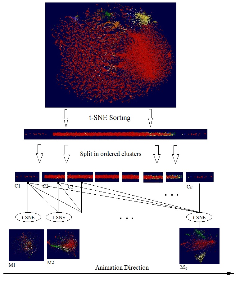
The t-SNE algorithm with the high fidelity modification offers a simple yet effective way to discover global sequential structure in high dimension data: we simplify apply t-SNE to reduce a given dataset  to 1-dimensional space. The coordinates of data points in the 1-dimensional space then provide the keys to order data points. The following video clip illustrates how t-SNE works on the dataset mentioned above:

We notice in above video that t-SNE discovered, more or less, the sequential structure underlying the sub-clusters; and furthermore, those partial sequential structures are aligned/ordered in a coherent way.

Dual Sorting of Heatmaps

Heatmap is a popular method to visualize matrix of numerical data. Heatmap is often used together with dendrograms, which rearrange the rows and columns using certain hierarchic clustering algorithm. The following picture shows a typical heatmap together with two dendrograms:

Heatmap augmented with dendrograms (wikipedia)

Heatmap constructed with dendrograms offers intuitive visualization, but it has difficulty to scale up to large dataset. For large matrix like those from single cell RNA sequencing (scRNA seq) study, dendrogram become quite inefficient, and instable in the sense that small change in data might lead to large variation in the clustering structure.

The t-SNE based sorting algorithm described in this note provides a simple alternative to arrange rows and columns in a heatmap: we simply sort the rows and columns with t-SNE. As an example, I took a dataset from scRNA Seq analysis, it comprises the gene expression counts of about 11000 cells with respect to 28000 genes. The following pictures shows its t-SNE embedding and its heatmap:

In above heatmap, each row represents the expression profile of a cell with respect to all selected genes; and each column represents the expression profile of a gene with respect to selected cells. Dark or red elements in the heatmap represent highly expressed cell/gene pairs. The t-SNE map is a embedding of all cells. We can see that several cell clusters are clearly visible as dark horizontal strips. However, no clear gene clusters are visible in the heatmap.

The following picture shows the heatmap after sorted its rows and columns with t-SNE. We see much more clearly the clusters among cells and genes, and more importantly the association between the  cell- and gene-clusters.

It should be noticed with regards to the experiment above:

• The perplexity of the t-SNE is set to about 2500. Smaller perplexity often leads to instability and random artifacts.
• The training process with t-SNE has ran for 5000 epochs, which is much higher than normal t-SNE training process. Training less epochs likely results in more random artifacts.
• In above example, t-SNE used the linear correlation as distance metric instead of the normally used Euclidean distance. Various experiments indicate that correlation seems to be more appropriate to measure similarity between genes. Because of this, we can not use PCA to pre-process data table to much lower dimensions to speed up the training, since PCA in general doesn't preserve correlation table.

Unfolding of t-SNE Embedding

We have previously blogged about doing "knockout" test with t-SNE. By comparing the t-SNE maps produced by the different set of genes, we can explore the impact of disabled genes. Going one step further, with t-SNE as a multidimensional sorting algorithm we can perform the following experiment:  We first sort all the participated genes into a sequence; then pick a particular direction for the sequence and split the sequence in small clusters; then create t-SNE cells maps with progressively larger gene clusters.  The following diagram illustrates these steps:

It should be noticed that the sequence of t-SNE maps are generated independently by separate training processes, and each of them started from a different random initialization. In other words, the final maps M1, M2, M3 are independent embeddings of ordered gene clusters, C1, {C1, C2}, {C1, C2, C3}, etc.. If we are lucky, the order underlying the gene clusters might indicate certain latent variables, like time. The following short video clip shows the animation of through the resulting t-SNE maps for the dataset in previous section.

It is interesting to notice that the animation is reminiscent of  group of cells unfolding, generation by generation, to final shape and structure.

High Fidelity t-SNE

 High Fidelity t-SNE with Gradual Diminishing Exaggeration

When we repeat t-SNE on the same dataset with the same parameters, we may get different maps with noticeable random variations.  This kind of randomness limits the accuracy of t-SNE algorithm as a visualization tool.

In this note we describe a simple yet effective method to improve the accuracy of t-SNE: Instead of switching the exaggeration rate at a fixed time during the training, we propose starting the training process with a high exaggeration, say 12.0, then gradually reduce it to 1.0.  We will demonstrate the effectively of this method with example from single cell RNA sequential study.

Post-Training Normalization

Since the cost function optimized by t-SNE is invariant under rigged transformations (i.e. rotations and shifting), t-SNE normally produced maps with random rotations and shift. These kind of randomness can be easily removed by post-training normalization. For this study, we propose the following steps to normalize t-SNE maps as illustrated in the following diagram with 4 sample t-SNE maps:

As shown in above diagram, a t-SNE map is normalized in 3 steps:

1. Centralizing: centralizing the map so that each of the 2D or 3D coordinate has zero-mean.
2. PCA based Alignment: Rotating the map, so that the x-axis aligns with the first eigen vector of the map; y-axis with the second eigen vector, and potentially the z-axis with the third eigen vector.
3. Moment based Flipping: Calculate the 0.5-th moment of the map along the x-axis according the following forms: 
   
   
   
   If the moment is negative, flip the map along the x-axis by multiple all x components with -1.0;
   Do the same with y-axis and potentially z-axis.

After normalization we can then measure the discrepancy between two t-SNE maps by summing up the Euclidean distances between the data points in both maps. For more convenience, we can just count number of the data points whose images points have distance from each other larger than certain values, say 40 pixels.

It should be pointed out that there are cases that the suggested method might fail. For instance, when the t-SNP maps are rotational symmetrical where no clear orientation is present, this method will have difficulty find common orientations. In the practice, we often encounter this case, when the perplexity parameter of t-SNE is too small, so that the resulting t-SNE map resemble a disc or a ball. Fortunately, this kind of issue can be easily fixed by increasing the perplexity.

Finally, it is interesting to notice that there is no need to scale the maps, since t-SNE with fixed parameter settings normally produces maps with roughly the same size.

Training with Gradual Diminishing Exaggeration

In order to improve the training speed and efficiency, t-SNE algorithm initially proposed to start the training with a high exaggeration factor, train the map for certain number of epochs; then switch the exaggeration factor to 1.0 to practically terminate the exaggeration phase. The following diagram shows the cost minimized during a typical t-SNE training process, the diagram has been overplayed with the exaggeration factor.

We see that the objection cost has been reduced rapidly for a short period after the exaggeration phased has ended, but then stayed basically unchanged during the rest of the training process. This behavior suggests that real learning only takes place when exaggeration factor changes. We propose thus the following function to gradually decrease the exaggeration factor:

In above formula,  f(n) is the exaggeration factor at n-th training epoch; C is the initial exaggeration factor; N is the number of total training epochs; L is the length of exaggeration phase which is set normally to 0.9N. 

Example 

As example I picked a dataset from single cell RNA sequence (scRNA seq) study. The dataset contains the expression counts of about 22000 cells with respect to 28000 genes. The input data for the t-SNE is thus a 22000x28000 matrix. The following picture shows a heatmap and a t-SNE map of this dataset:

For the test, t-SNE has been run on the dataset 4 times with and without enabling the new exaggeration method. The following pictures shows the cost reduction during training of the four repeats:

We see that, with the new method enabled, the final t-SNE maps have consistently lower cost. We also notice that, with the new method, the final maps have almost equal costs, whereas with old method, the cost of final maps vary slightly. Those small variations are more visible in the final maps. The following two pictures show the maps created with and without the new method:

With some effort we can discern relative large variation amount the maps created with old exaggeration strategy. We can visualize those variations more clearly with animation by interpolation between those maps as be shown in the following video clip:

Knockout Test with High Fidelity t-SNE

Knockout test has been used in microbiology to probe gene functions during the development of organisms. For doing that, certain genes are disabled or knocked-out; and changes induced in the organism give indications about those knocked-out genes.  In general, knockout test help us to trace the correlation between genotypes and phenotypes.

High fidelity t-SNE enables us to probe the effect of individual features on the output t-SNE maps. If consider the t-SNE maps as phenotypes derived from genotypes (i.e. gene expressions), we can perform kind of "knockout" test with t-SNE:  We create first a t-SNE map with all features; then create a t-SNE  map without certain features. We can then expect that the knocked out features would be responsible for the variation in the t-SNE maps.

The following short video demonstrates how "knockout" test might been done to study correlation between gene- and cell-clusters:

Conclusion

With a small change in its algorithm, t-SNE achieved much high accuracy and opens therefore doors for new applications.