On Multidimensional Sorting

In a previous blog post I have talked about a method to convert photos to high dimensional datasets for analysis with MDS methods. This post will address the opposite problem: given a high dimensional dataset, can we convert it to a photo alike 2D image for easy feature recognition by human?

Let's consider our sample dataset S&P 500. A direct approach to create a 2D map is to simply convert the matrix of real values to a matrix of gray-scale pixels. This can be easily done in VisuMap with the heatmap view and the gray-scale spectrum. The following picture shows the S&P 500 dataset in normal line diagram view on the left side and the corresponding heatmap on the right side:

Each curve in the left picture corresponds to the price history of a S&P-500 component stock in a year. We notice heavy overlaps among the curves. On the right side, the heatmap represents the stock prices with row strips with different brightness. In the heatmap, we can spot roughly the two systematical downturns at the two slightly darkened vertical strips. There is however no discernible pattern between the rows, as the rows are just ordered by their stock ticks, so that neighboring relationship don't indicate any relationships between their price history.

One simple way to improve the heatmap is to group stocks with similar price history together. This is the task of most clustering algorithms. We can do this pretty easily in VisuMap. The following heatmap shows the same dataset after we have applied k-Mean clustering algorithm on the rows and re-shoveled the rows according to cluster assignments:

The k-Mean algorithm has grouped the rows into about 8 clusters, we can see that rows within each group represent rows with, more or less, similar values. However, the clusters are randomly ordered, and as well as the rows within a cluster. The clustering algorithm does not provide ordering information for individual data points.

Can we do better job than the clustering algorithm? To answer this question, let's recall what we actually tried to do above: we want to reorder the rows of the heatmap, so that neighboring rows are similar to each other. This kind task is basically also the task of MDS (Multdimensional Scaling) algorithms, which aim to map high dimensional data to low dimensional spaces while preserving similarity. Particularly in our case, the low dimensional space is just the one-dimensional space, whereas MDS in general have been used to create 2 or 3 dimensional maps.

Thus, to improve our heatmap,  we apply a MDS algorithm to our dataset to map it to an one-dimensional space, then use their coordinates in that one-dimensional space to re-order the rows in the heatmap. For this test, I have adapted the RPM mapping (Relational Perspective Map) algorithm to reduce the dimensionality of the dataset from 50 to 1, then used the one-dimensional RPM map to order the rows in the heatmap. The following picture shows a result heatmap:

We notice this heatmap is much smoother than the previous two.  In fact, we can see that the data rows gradually change from bright to dark color, as they go from the top to the bottom. More importantly, we don't see clear cluster structure among the rows, this is in clear contrary to the k-Mean algorithm that indicates 8 or 10 clusters. In this case, it is clear that k-Mean algorithm delivered the wrong artificial cluster information.

Now, a few words about the implementation. The multidimensional sorting has been implemented with RPM algorithm, since RPM allows gradually shrinking the size of the map by starting with 2D or 3D map. This special feature enables RPM to search for optimal 1D map configuration among a large solution space. We could easily adapt other MDS algorithms to perform multidimensional sorting, but we probably will have to restrict solely on one-dimensional space with those algorithms. A few years ago, I have already blogged about this kind of dimensionality reduction by shrinking dimension with some simple illustrations.

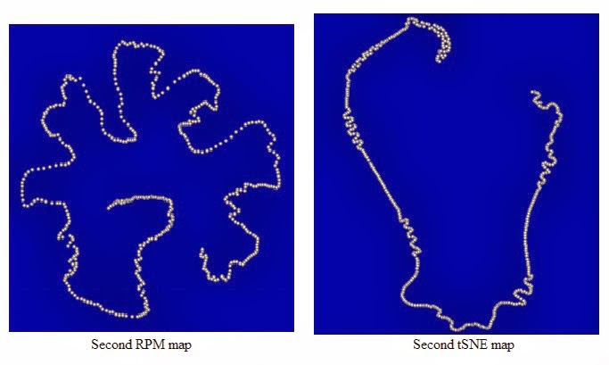
Since high dimensional datasets are generally not sequentially ordered, there are in general not an unique way to order the data. What we want to do is just find a solution that preserves as much as possible similarity information with the order information. Thus, an important question arises here: How do we validate the sorting results? How do we compare two such sorting algorithms?  A simple way to validate the sorting result is illustrated in the following picture:

So, in order to test the sorting algorithm we first take simple photo and convert it to high dimensional dataset that represents the gray-scale levels of the photo. We then randomize the order of the rows in the data table. Then, we apply the sorting algorithm on the randomized data table, and check how good the original photo can be recovered. I have done this test for some normal photos, the multidimensonal sorting was able to recover pretty well the original photo (see also the short attached video), as long as enough time is given to the learning process.

We have described an application of MDS algorithm for heatmap by using it to reduce data dimension to a single dimension. We might go a step further to use MDS to reduce data dimension to 0, so that data points will be mapped to a finite discrete points set. In this way, we would have archived the service of clustering algorithms. If this works, clustering algorithms can be considered a special case of MDS algorithms; and MDS algorithms might lead us to group of new clustering algorithms.

The multidimsional sorting service has been implemented in VisuMap version 4.0.895 as integrated service. The following short video shows how to use this service for the sample datasets mentioned above.

A more practical application of MDS sorting is for microarray data analysis where heatmaps are often used to visualize the expression levels of a collection of gens for a collection of samples. Normally, neither the gens nor  the samples are ordered according to their expression similarity, so that those heatmaps often appear rather random (even after applying additional grouping with hierarchical clustering algorithm.) The following picture shows, for instance, a heatmap for expressions of 12000 genes for about 200 samples:

After applying MDS sorting both on the rows and columns of above heatmap, the heatmap looks  as following:

The above heatmap contains theoretically the same expression information. But, just by re-ordering the rows and columns, it shows more discernible structure and information for human perception.

VisuMap version 4.0.895 released

We have just released VisuMap version 4.0.895. The following is a list of major changes:

• Implemented the multidimensional sorting and on-fly mapping & clustering services.
• Extended the RPM algorithms with dark-pressure mechanism.
• Reduced memory usage of the application significantly, so that it can load much large dataset.
• Various defect fixing and enchantments

On the shape of pictures

This blog post is going to talk about a simple way to convert normal 2D pictures or photos to high dimensional datasets; and then use MDS tool to analyze those data. At the end, I'll mention some potential uses of this type of analysis for data from practical cases.

Assuming that we have a picture that is represented by a MxN matrix of pixels, The pixel matrix can be simply converted to a matrix of real numbers by replacing each pixel with its intensity (or brightness) using the formula: a = 0.114*R + 0.587*G + 0.299*B; where R, G, B are the red, green and blue intensities of the pixel. We consider this MxN matrix as a N-dimensional dataset with M data points, where each data point is just a row vector in the matrix.

Obtained such a high dimensional dataset for our picture, we can then visualize this dataset with various MDS methods. The following picture shows visualizations of a sample photo with three different MDS methods, namely, PCA, tSNE and RPM:

We see that all three methods reveal, more or less, a serial structure among the data points (i.e. rows in the pictures.) When using MDS methods to visualize high dimensional data, the first question we ask is often: Are the maps reliable? Asked differently, Do those geometrical shapes in maps show some nature of the initial dataset, or are those shapes just random result of those algorithms? To answer this question, I have run RPM and tSNE multiple times, all runs produced, more or less, similar maps (the PCA algorithm is deterministic, will therefore always produce the same 2D map.) The following picture shows two more maps produced by RPM and tSNE algorithms:

Comparing above two pictures we see that both RPM and tSNE algorithms produced repeatable results by different runs despite their non-deterministic nature. Going one step further, we could ask what kind maps we'll get when we alter the sample dataset slightly. To answer this question, I have created a RPM map and a tSNE map with half of the rows and half of the columns by chosen alternately each other row and column of the matrix (i.e. only with 1/4 of the data matrix). The following picture shows the result maps:

Above maps show apparent similarity with the maps in previous picture. Thus, we have here strong evidence that the geometrical characteristics in these maps correlate with characteristics in the initial sample picture. We can see such correlation more clearly when exam how regions of the map represent sections in the sample picture. The following picture shows how some sections of the tSNE map correspond to sections in the sample picture:

We notice that MDS maps topologically have simple sequential structure, so no information are embedded into the topological structure. MDS maps rather carry information through geometrical characteristics. For instance, a section of smooth curves; a large arch; a section of points with less density; etc.;  Also, two distant sections winding together in particular way may indicate special feature of the underlying data. Furthermore, when we use 3D MDS maps, those secondary structure over the sequential structure may reveal much more rich complex information about the high dimensional data. Thus, MDS maps may offer new ways to describe and analyse the initial picture.

We might ask here: why are the MDS maps of the picture sequential?  To answer this question, let's image that we scan the picture from top to bottom, line by line, and store the line in a vector, then this vector will gradually change from one line to the next line. Thus, this line vector manifest a kind random-walk in the high dimensional space mostly with relatively small steps. Those random-walk alike datasets exist in many areas of data analysis. For instance, a while ago I have blogged about one such case where the state of the whole stock market has been considered as an random-walk process. We notice also that the MDS maps shown above resemble, more or less, those map in the blog self-similarity of high dimensional random-walk.

The following picture shows the price history of  S&P 500 components for a year, and the corresponding RPM map where each dot represents the state of the stock market at a day:

We notice the apparent similarity of the above RPM map with that produced for our sample picture previously. Thus, notions and methods developed for analyzing pictures may apply to a broader scope of data.

One interesting question arises in view of above picture is: Can we produce 2D picture (maybe not as nice as the photo of Lena but with easier recognizable features) out from a high dimensional dataset like the S&P 500 dataset? The answer is pretty much positive, and I'll blog about this in another post where I will talk about about multidimensional sorting.

At last, the sample picture and maps in this blog is produced by VisuMap version 4.0.895 and the sample dataset can be downloaded from the link here. The following short video shows some basic steps to apply mentioned services:

Visual Data Cleansing with VisuMap

I have just uploaded a short video (7min) that demonstrates how to do data cleansing visually with VisuMap. The sample dataset used in the video can be downloaded from here.

Sorting high dimensional data with RPM maps

I have recently published a dataset  that contains the daily prices of the S&P 500 component companies for a period of 5 years. The mountain view of VisuMap provides a pretty good overview of the whole dataset in 3D styles. The following short video clips shows the normalized values (so that all price history start from 1.0) of the dataset:



We notice that the curves are colored using the k-Mean algorithm, so that stocks with similar development will have common colors. However, these curves are not ordered according to their group, but according to the alphabetic order of the stock tick, so that curves of different colors are all mixed with each other.

A simple way to enhance the 3D view is just to re-order the curves, so that curves of the same group will be located together. We can do this easily with the heat-map view of VisuMap. However, this method does not reorder the groups in a meaningful way, so that closely located groups, are not necessarily similar groups.

The RPM map provides a better way to sort high dimensional data according to similarities. To do this with VisuMap, we first create 3D RPM map for the dataset with very large width (e.g. 1200 pixels) but small height and depeth (e.g. 50 pixels), so that RPM map geometrically resembles a ring. Then we sort the  data points according to the x-coordinates in the 3D RPM map ( that determines the data point's position on the ring.) The nature of the RPM algorithm will make sure that closely located data points on the RPM map will be similar to each other.

The following short video shows how to do this with VisuMap. Notice that we have already created the 3D RPM map. To reorder the data points, we opened a table for the XYZ coordinates, then sorted the table on the X-coordinate column. The mountain view has been configured to automatically re-order its content when re-ordering-event occurred.

Daily Price of S&P Companies in last 5 years.

I have just released a new VisuMap dataset that contains the daily prices of S&P 500 companies for the year 2008 to 2012. This dataset, available at our web site, provides convenient access to these stock prices for that period. The dataset also contains scripts which download automatically those historical data from Google server.

The following is short video to display these data in 3D mountain view:

Visual interface kNN data clustering services in VisuMap

I have just uploaded a short video tutorial (ca. 10 minutes) that demonstrates the visual interface for the kNN (k-nearest neighbors) data clustering service in VisuMap version 4.0.892. The tutorial shows, with two scenarios, how to combine kNN with supervised and unsupervised classification methods.

Although kNN has been one of the simplest and most widely used classification algorithm, there is no software on the market that provides kNN services with decent visual interface. VisuMap implemented a unique visual interface for kNN with the help of MDS mapping and linked data views.

Azhimutal projection for RPM on projective spaces

Among those manifolds used by relational perspective map (RPM), the 2-dimensional real projective plane (P2) has been one of my favorite space. As a visualization space for high dimensional data, P2 works similarly as the 2-dimensional flat torus (T2) used initially by RPM.  Both T2 and P2  provide a boundaryless view of data by connecting the opposite sides of the space. Both spaces are completely isometrics and shifting/rotation symmetrical.

P2 has, however, one advantage over T2 in that P2 is isotropic but not T2. This means that P2 is equivalent in all directions, but T2 treats different directions differently. For instance, the diagonal directions of T2 usually aligns with the larger portion of the data as I blogged about this before. P2 doesn't have such space specific artifacts: P2 maps are usually symmetric in all direction and can be rotated freely.

On the other side, T2 do have a significant advantage over P2 as it a flat but not P2:  T2 maps are represented as rectangular maps whereas P2 maps are maps on the semi-sphere. This makes P2 maps harder to explore on conventional flat media like paper or computer screen. VisuMap has implemented a special sphere view to facilitate the exploration of spherical maps, but the rectangular T2 maps are still fare more easier to explore than the sphere view.

The problem to represent spherical surface through flat map is, of course,  a quite old problem. A plethera of methods have been invented in the past to create flat maps for the spherical earth surface. Looking in to method list at the page Map Projection, I have picked the Azhimutal projection to project the semi-spherical P2 maps to the flat plane. This additional projection has been implemented in the latest version of VisuMap 4.0.892 with which you can make disk-like snapshot of a spherical P2 map in the sphere view. The following picture illustrates how VisuMap maps data from high dimensional space to P2 and then to the flat plane with the Azhimutal projection:

We notice that the Azhimutal projection is a non-linear project, it will stretch the area a the boundary of the semi-sphere somewhat. This kind of non-linear stretch will mathematically induce non-zero curvature on the flat disk, so that the total curvature of the stretched disk equals that of the semi-sphere (as the Gauss-Bonnet theorem dictates.) The following short screen-cast shows how VisuMap maps the full sphere on the the semi-spherical P2 space. The RPM algorithm will split the sphere into 4 pieces. Notice how these fragments stretch when rotating them from center to the boundary.

Going one step further, we have extend the Azhimutal projection to project 3-dimensional projective space (P3) to the 3D flat space where P3 is realized as a semi-sphere in 4-dimensional space. In VisuMap, such a 3D map is called a projective ball (where the opposite points on the surface have been considered stuck together.) The following screen-cast shows how VisuMap creates RPM-3P map for the S&P 500 dataset:


Notice that the RPM 3P actually resides in the 4D space. We have developed a special view that in addition to rotation among the first three dimensions, also allows rotation between the first 3 dimensions and the forth dimension (active when pressing-and-holding the control-key.)

On the weighted Hamming distance

Hamming distance is a simple distance function to impose a metrical structure over discrete non-numerical data. Hamming distance has been widely used to cluster or visualize discrete data. In VisuMap Hamming distance has been so fare the only distance function for discrete date. In this note I'll introduce the weighted Hamming distance (WHD) as an extension to the Hamming distance. After a brief review of the original Hamming distance, I'll describe WHD and demonstrate its strength with two sample datasets.

Let's first consider the one-dimensional case. Let Ω be a set of data points potentially with duplicates. Ω may represent, for instance, the hair color or blood type of a group of patients. The Hamming distance between two data points x and y is simply defined as:

The weighted Hamming distance (WHD) is defined as:

where p(x) is the frequency of the value x in Ω.  |Ω| is the number of data points in Ω. w(x,y) is an extension of d(x,y) in the sense that d(x, y) < d(x', y') always leads to w(x, y) < w(x',y'). On the other side, w(,) is actually not a distance function in strict terms of mathematics, since w(,) does not fulfill the requirement w(x,x) ≡ 0.

We notice that d(,) takes the value 0 and 1, whereas w(,) can take any value from 1 to |Ω|. d(,) only captures the information about equality, whereas w(,) captures, in addition to the equality, also the frequency of each different discrete value. In particular w(x,y) yields smaller distance if the value x is infrequent in Ω. In terms of our example with patients as data points, w(,) will ascribe larger closeness (i.e. smaller distance) to a pair of patients if they share a rare property values, say a rare blood type. This property of WHD make it to focus more on rare property values.

In multidimensional case, our data points will be assumed to be from a multidimensional space x = (x₁, x₂...x_n)∈Ω₁×Ω₂×...×Ω_n; Let y = (y₁, y₂...y_n) be a second the data point; and let w_k be the weighted hamming distance between x_k and y_k; then we define the multidimensional WHD between x and y as:

We notice that the multidimensional WHD is, up to a constant factor, the harmonic mean of weighted hamming distance of each individual dimension. The harmonic mean, like the normal arithmetical mean, yields a number between the minimal and maximal value in {w₁, w₂, ..., w₃}, except that the harmonic mean is normally shifted towards the minimal value. The use of harmonic mean instead of the squared sum (as used by Euclidean distance) makes w(,) bias towards smaller values in the set {w₁, w₂, ..., w_n}. This means, in terms of our example with patient data, we ascribe more importance to those properties which show larger proximity between data points. For instance, if the hair color property are more or less randomly distributed among the patients, but some specially blood types occur only rarely, then the blood type property will be more importance with respect to the harmonic mean.

To see the difference between WHD and normal hamming distance we first consider the sample dataset Adult Database in the UCI Machine-Learning repository that collects information about students. For the sake of simplicity I just use two properties, education and race, to generate MDS maps. The following are the MDS maps generated with CCA mapping algorithm with WHD and normal hamming distance, on the left and right side respectively:

In above picture we can see clearly in the left map that three large clusters occupy the whole data space, whereas the left map only show a cloud with discrete data points without visual information about the cluster sizes.

As second example we consider a dataset in Haplotype Analysis. This dataset contains about 2000 data points each comprises the haplotypes of about 160 SNPs. The following picture shows the MDS maps generated with the tSNE algorithm with WHD and normal Hamming distance, on the left and right side respectively:

We notice that map on the left side reveals about 8 clusters with different sizes, whereas the map on the right side (generated with Hamming distance) shows four, more or less, symmetrical clusters. The map generated with WHD shows more structure and complexity, but is up to the scientist to verify the relevance of those extra structural information.

Weighted hamming distance has been implemented in VisuMap 4.0 as a new metric for enumerated data. The above sample maps are generated with VisuMap version 4.0.891.

VisuMap 4.0 Released

We have just released VisuMap 4.0 with new price list for our software products and services. This release is a major upgrade from its previous release v3.5 (released about two years ago). Main changes in this release include:

• Upgraded the .Net Runtime library from version 2.0 to 4.0. Some new features in the .Net 4.0 significantly simplified internal implementation and most likely also improved the performance and stability. For example, the support for generic covariant list greatly speeded up a lot data processing.
  
• Implemented new services to analyze tables with non-numerical data.. We have for instance introduced the weighted-hamming distance to geometrize multidimensional enumerate data. These features manifest our R&D in the past year that moved gradually towards analysis of non-numerical data. We'll talk about this simple and interesting metric in latter blogs.
  
• We have increased the price for our products and services for 10% to 15%. This is the first price increase in last two years. 

For more information about VisuMap 4.0 please see the "What's new" section in the product's on-line help and our web site.