One sample dataset distributed with the VisuMap software package is the normalized weekly stock price history of 500 S&P stocks for the year 2002. This dataset as shown in the following picture can be considered as 500 time series for about 50 time points (i.e. weeks).

Picture 1
While above picture shows some common trend (like the large downturn in middle of the year), the price development is predominately random. How can we characterize this randomness? Well, one way to model the randomness is considering the stock price developments as independent random walk processes: Assuming that you have invested one dollar in each of the 500 stocks, their values will change more or less randomly from week to week for a small percentages. As a reference model we can generate 500 such random walk process with the following JavaScript code (as supported by VisuMap):
var randomWalk = New.NumberTable(500,50);The last line in above code block creates the following diagram (the diagram has been colored with k-mean algorithm):
for(var row=0; row < randomWalk.Rows; row++) {
var v = 1.0;
for( var col=0; col < randomWalk.Columns; col++) {
randomWalk.Matrix[row][col] = v;
v *= 1 + 0.01*(Math.random() - 0.5);
}
}
randomWalk.ShowValueDiagram();

Picture 2
Comparing Figure 1 and 2, we can say that Figure 2, more or less, resembles Figure 1 if we remove some common trends from Figure 1 (i.e. de-
trending the down-turn in the middle and the overall slightly down-wards trend). The resemblance is however a collective similarity. It
does not make sense to find similarity between individual curves in the two figures.
Another way to compare two sets of time series is using principal components analysis (PCA). Among many other services, PCA provides a systematic way to decompose high dimensional variances in a dataset into many 1-dimensional directions. These directions (called principal components) are also ordered in the way, so that the beginning components have larger variance and therefore more information. Thus, PCA might be interesting way to characterize the variance (i.e. some kind of randomness) in a dataset.
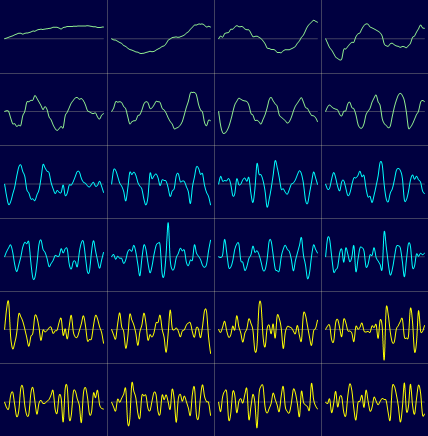
It is very simple to visualize the PCA components with VisuMap. To do so, we just need to open the PCA view and open the Projection Analyzer window. Then select some PCs and choose the context menu "Show PCAs". The following two picture shows the first 24 PCs of the S&P500 and the RandomWalk datasets:
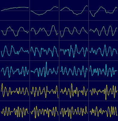 Picture 3
 Picture 4
We can clearly see some similarity between the first few PCs in above two pictures. This indicates that random walk process models pretty well the major variance directions of the S&P dataset. The discrepancy between the PCs in above two picture may be used to characterize how the S&P price history differs from random walk process. In this way the random walk process is used as a null-space reference model.
Looking at Picture 4 we can also notice an interesting thing: the PCs clearly resembles the curves of sine functions. This is actually not too surprising since the PCA algorithm is basically a sequence of high dimensional rotation operations, which, as we know, lead to a lot of sine/cosine functions. Nevertheless, it would be interesting to determine the exact mathematical formula for the random walk process. By doing so, we can have a quick statical approximation for PCAs of many random walk alike datasets.
It is very simple to visualize the PCA components with VisuMap. To do so, we just need to open the PCA view and open the Projection Analyzer window. Then select some PCs and choose the context menu "Show PCAs". The following two picture shows the first 24 PCs of the S&P500 and the RandomWalk datasets:
 Picture 3
 Picture 4
Looking at Picture 4 we can also notice an interesting thing: the PCs clearly resembles the curves of sine functions. This is actually not too surprising since the PCA algorithm is basically a sequence of high dimensional rotation operations, which, as we know, lead to a lot of sine/cosine functions. Nevertheless, it would be interesting to determine the exact mathematical formula for the random walk process. By doing so, we can have a quick statical approximation for PCAs of many random walk alike datasets.
No comments:
Post a Comment